
 EN
EN JA
JA

TL;DR — Key Takeaways
- The Transformer converts text tokens into rich, context-aware numerical representations.
- Self-Attention lets every word simultaneously communicate with every other word — no sequential processing.
- Multi-Head Attention runs attention from multiple perspectives in parallel, capturing grammar, meaning, and references at once.
- The Encoder stacks N layers of Attention + Feed-Forward blocks, with Residual Connections and Layer Norm for stability.
- This approach replaced RNNs because it parallelises computation and handles long-range dependencies effortlessly.
The Big Picture
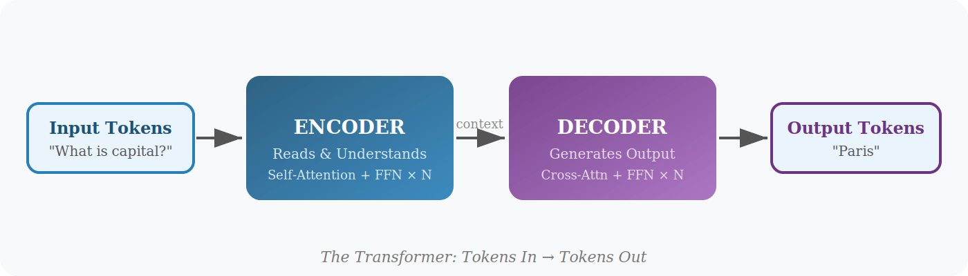
A Transformer is, at the highest level, a tokens-in, tokens-out machine. Feed it a sequence of tokens and it produces a sequence of tokens. Everything else — the attention heads, the layers, the embeddings — exists to make that mapping as powerful as possible.
Why Was the Transformer Needed?
Before Transformers, sequence models processed words one by one — left to right, in order. Two fundamental problems plagued them.
Forgetting. As sentences grew longer, early words faded from memory. By the time the model reached word 50, word 1 was nearly gone.
Slowness. Sequential processing meant each word waited for the previous one. No parallelism, no speed.
What Came Before: RNNs, LSTMs, and GRUs
Three architectures dominated the pre-Transformer era, each an improvement on the last.
RNN — The Forgetful Storyteller
An RNN reads words one at a time, keeping a “hidden state” — a running memory of what came before. The trouble: as sequences grow longer, early information vanishes. In the sentence “The cat chased the mouse because it was hungry,” an RNN reaching “it” has often already lost clear memory of “cat.” This is the vanishing gradient problem.
LSTM — The Note-Taking Storyteller
LSTMs added a cell state — like a notebook — controlled by three gates: a Forget Gate (should I drop this?), an Input Gate (what new info matters?), and an Output Gate (what do I need right now?). This selective memory solved the vanishing gradient problem for most practical sentence lengths.
GRU — The Efficient Storyteller
GRUs simplified the LSTM’s three gates into two (Update and Reset), combining the cell and hidden states. Fewer parameters meant faster training with comparable performance. But all three architectures shared the same bottleneck: sequential processing.
| Architecture | Memory Style | Strength | Weakness |
|---|---|---|---|
| RNN | Single running state | Simple, fast | Forgets long sequences |
| LSTM | Gated cell + hidden state | Long-range memory | Slow to train |
| GRU | Combined gated state | Fast + effective | Still sequential |
| Transformer | Full attention over all tokens | Parallel, any range | Needs more data |
The Architecture Has Two Halves
The original Transformer splits into two complementary components. The Encoder reads the full input and builds a rich contextual understanding of every token. The Decoder uses that understanding to generate output, one token at a time.
Step 1: Turning Words into Numbers
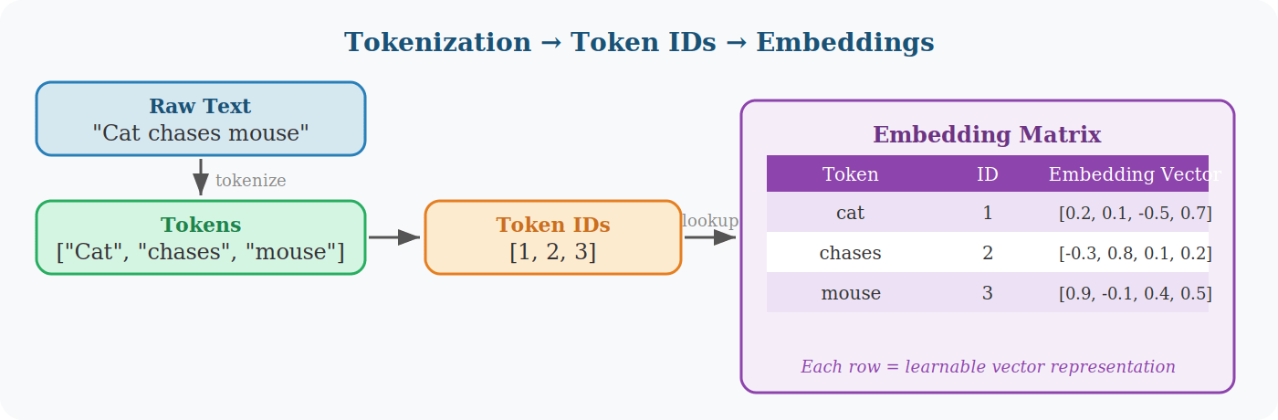
Computers understand numbers, not words. Before any attention mechanism can run, the input text must be converted into numerical representations. This happens in two stages: tokenization and embedding.
Tokenization
The tokenizer splits raw text into units called tokens. A token might be a whole word, a subword piece, punctuation, or even an emoji. For clarity, this guide treats each word as one token.
“Cat chases mouse” → [“Cat”, “chases”, “mouse”] → Token IDs: [1, 2, 3]
The tokenizer maintains a vocabulary — a giant dictionary mapping every known token to a unique integer ID. The ID itself carries no meaning; it is merely a position in a lookup table.
| Model | Vocabulary Size |
|---|---|
| BERT | S~30,000 |
| GPT-2 | ~50,000 |
| LLaMA | ~128,000 |
Embeddings — The Semantic Fingerprint
Token IDs get looked up in an Embedding Matrix — a learned table where each row is a dense vector of floating-point numbers representing one token. These vectors are not hand-crafted; they are learned during training and encode semantic meaning: similar words end up with similar vectors.
| Model | Embedding Dimension |
|---|---|
| Small models | 128 |
| BERT Base | 768 |
| GPT-3 | 12,288 |
The Library Analogy
Think of the vocabulary as a library catalog and each token ID as a shelf number. The shelf number tells you where to find a book — but the book’s actual content (plot, characters, themes) is the embedding vector. The model learns richer and richer “book content” throughout training.
Step 2: Adding Word Order — Positional Encoding
Unlike RNNs, the Transformer processes all tokens simultaneously. This is its great advantage — and its problem. Without extra information, “Dog bites man” and “Man bites dog” contain identical tokens and would be indistinguishable.
The fix is positional encoding: a mathematical signal added to each embedding that encodes where in the sequence that token sits. The original Transformer uses sine and cosine waves at different frequencies to generate these signals.
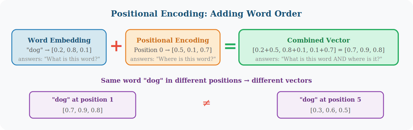
Key insight: The word embedding answers “What is this word?” — the positional encoding answers “Where is this word?” — the combined vector answers both simultaneously.
Step 3: The Attention Mechanism
This is the heart of the Transformer. Attention allows every token to simultaneously look at every other token and decide how much focus to give each one — all in a single parallel operation.
When the model reads “it” in “The cat sat on the mat because it was tired,” attention lets “it” check all other words and determine — from the pattern of relationships — that it refers to “cat,” not “mat.”
Query, Key, and Value
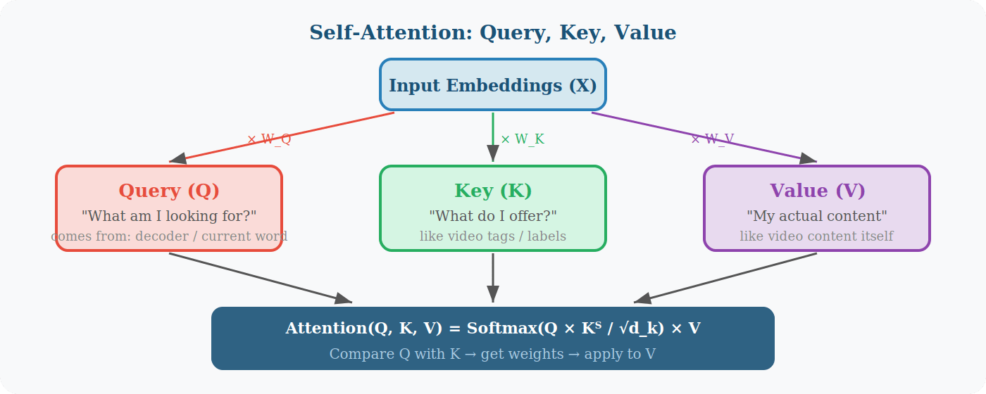
Each token is projected into three vectors using learned weight matrices:
- Query (Q): “What am I looking for right now?”
- Key (K): “What information do I contain / offer?”
- Value (V): “What information should I pass along if selected?”
A useful analogy: when you search YouTube, your search query is Q, each video’s title and tags are K (searchable labels), and the video’s actual content is V. YouTube matches your query to the most relevant keys, then serves you those videos’ content.
The Attention Formula
Attention(Q, K, V) = Softmax( Q × Kᵀ / √d_k ) × V
The formula in plain English: compute a similarity score between every Q-K pair (dot product), scale to prevent vanishing gradients (divide by √d_k), convert to probabilities (Softmax), then use those probabilities to weight-sum the Values. The result is a new representation for each token that blends information from all other tokens proportionally to their relevance.
Worked Example: “Cat Chases Dog”
Step 1–2: Input Matrix and Weight Matrices
Given embeddings for three words (dimension 4), we multiply the input matrix X by three learned weight matrices W_Q, W_K, W_V to get Q, K, and V matrices (dimension 3).
| Word | Embedding Vector |
|---|---|
| cat | [1.0, 0.0, 1.0, 0.0] |
| chases | [0.0, 1.0, 0.0, 1.0] |
| dog | [1.0, 1.0, 0.0, 0.0] |
Steps 3–6: Computing Attention Scores
| Step | Operation | Result |
|---|---|---|
| 1 | Q = X × W_Q | Q: cat=[2,0,1], chases=[0,2,1], dog=[1,1,1] |
| 2 | Scores = Q × Kᵀ | cat→chases scores highest (5 vs cat=1, dog=3) |
| 3 | Scale by √d_k = 1.73 | Prevents excessively large dot products |
| 4 | Softmax → probabilities | cat attends to chases 70.7%, dog 22.3% |
| 5 | Output = Weights × V | Each word representation blends context from all others |
After attention: “cat” now contains strong information about “chases.” “dog” also connects to “chases.” The model understands “cat is chasing dog” — not just three isolated words.
Step 4: Multi-Head Attention
Running attention once gives one perspective on token relationships. But language is rich — the same sentence simultaneously encodes grammar, semantics, coreference, and positional structure. Multi-head attention runs the attention mechanism several times in parallel, each with independent weight matrices, so each head learns different relationship patterns.
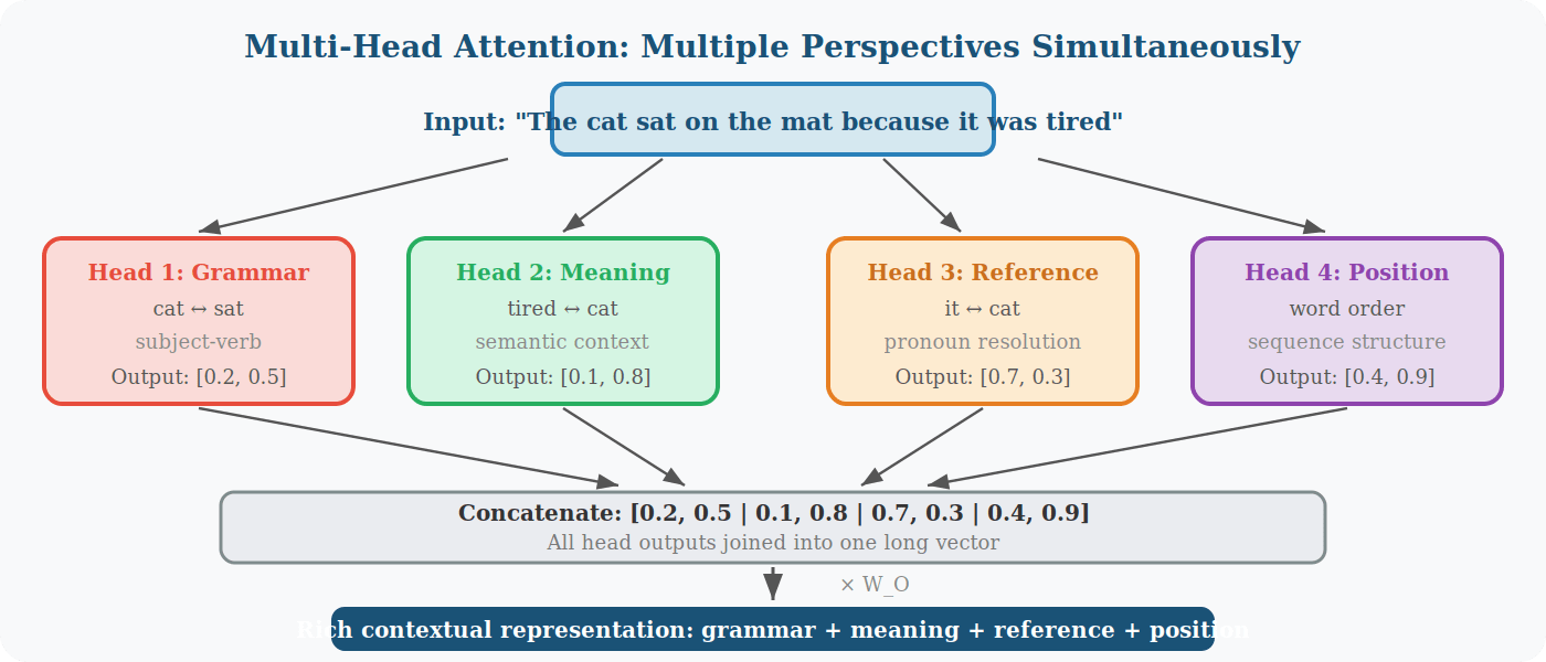
In the sentence “The cat sat on the mat because it was tired”: Head 1 might focus on cat ↔ sat (subject-verb), Head 2 on tired ↔ cat (semantic state), Head 3 on it ↔ cat (pronoun resolution), and Head 4 on positional structure. All four run simultaneously. Their outputs are concatenated and passed through a final linear layer W_O that combines all perspectives into one rich representation.
Step 5: Feed-Forward Network (FFN)
After attention has gathered context from across the sequence, each token’s representation passes independently through a Feed-Forward Network — two linear layers with a ReLU activation in between.
If attention is students discussing ideas together, the FFN is each student going home and refining their own notes. Attention determines which words matter to which; the FFN strengthens useful features and suppresses weaker signals, creating richer representations before the next layer.
Step 6: Residual Connections and Layer Normalization
Deep networks are difficult to train. Two techniques in every Transformer layer keep learning stable.
Residual Connection
Instead of passing only the transformed output forward, the Transformer adds back the original input:
Output = x + SubLayer(x)
This “skip connection” ensures that even if a layer learns poorly, the original information is preserved. It also dramatically improves gradient flow during training, enabling networks 96+ layers deep.
Layer Normalization
After each residual addition, values are normalised — shifted to have zero mean and unit variance. This prevents numbers from growing unboundedly across layers and keeps training smooth and stable. Together, residual connections and layer norm are what allow modern LLMs with hundreds of layers to train at all.
| Component | Purpose | Analogy |
|---|---|---|
| Residual Connection | Prevents information loss across layers | Keeping your original notes while adding teacher’s explanations |
| Layer Normalization | Stabilises value ranges | Standardising scores so they’re always comparable |
Step 7: Stacking Multiple Layers
One Transformer layer — one attention block plus one FFN, wrapped in residual connections and layer norm — is called a Transformer block. The Encoder stacks N such blocks sequentially. The output of block 1 feeds into block 2, and so on.
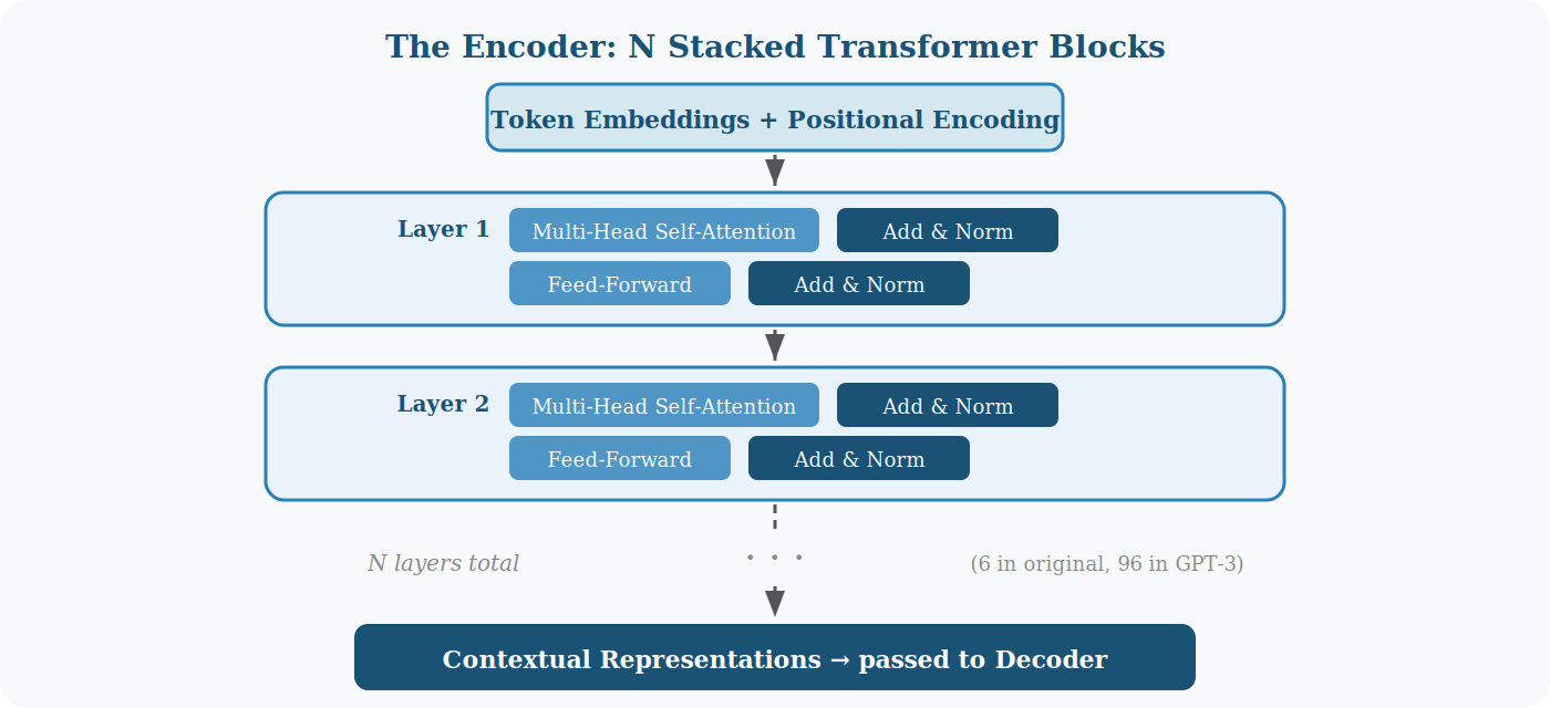
Think of each layer as reading the same sentence again but with deeper understanding each time. The first pass gives basic word meanings. The second reveals grammatical structures. The third captures semantic nuance. By layer N, representations are deeply contextual.
| Model | Encoder Layers | Parameters |
|---|---|---|
| ROriginal Transformer | 6 | ~65M |
| BERT Base | 12 | 110M |
| GPT-3 | 96 | 175B |
Summary: The Complete Encoder Pipeline
| Step | Component | What it Does |
|---|---|---|
| 1 | Tokenization | Split text into tokens; map to integer IDs |
| 2 | Embedding Lookup | Convert token IDs to dense semantic vectors |
| 3 | Positional Encoding | Add position signal so order is preserved |
| 4 | Multi-Head Self-Attention | Every token attends to every other token, multiple perspectives |
| 5 | Feed-Forward Network | Refine each token representation independently |
| 6 | Residual + Layer Norm | Preserve information, stabilize training |
| 7 | Stack × N | Repeat 4–6 for deeper understanding |
| Output | Contextual Representations | Passed to the Decoder for generation |
Frequently Asked Questions
What is a Transformer in artificial intelligence?
A Transformer is a deep learning architecture that processes text using self-attention, allowing every token to consider the context of all other tokens. It powers modern AI systems such as ChatGPT, Gemini, Claude, and many other large language models.
Are Transformers and Large Language Models (LLMs) the same ?
No. A Transformer is the underlying neural network architecture, while a Large Language Model (LLM) is an AI model trained on large datasets using the Transformer architecture. Most modern LLMs are built on Transformers.
What is the difference between Query, Key, and Value (Q, K, and V)?
Query represents what a token is looking for, Key represents the information each token offers, and Value contains the information passed to the output. Together, they enable the attention mechanism to identify and combine relevant context.
How do Transformers help Large Language Models understand language?
Transformers help LLMs understand language by combining embeddings, positional encoding, and attention mechanisms to capture context, identify relationships between words, and generate accurate, context-aware responses.

